그래프는 matplotlib로 그린다.
# 1. 데이터 전처리
from keras.models import Sequential
from keras.layers import Dense
import numpy as np
x = np.linspace(1, 10, 10)
y = x
# 2. 모델 구성
model = Sequential()
model.add(Dense(10, input_dim=1, activation='linear'))
model.add(Dense(10, activation='linear'))
model.add(Dense(8, activation='linear'))
model.add(Dense(1))
# 3. 모델 훈련
model.compile(optimizer='adam', loss='mse', metrics=['mae'])
model.fit(x, y, epochs=100, verbose=0)
# 4. 모델 평가 예측
loss_met = model.evaluate(x, y, batch_size=1)
print(loss_met)
predict = model.predict(x)
print('y', y, ' predict: \n', predict)
# RMSE 구하기
from sklearn.metrics import mean_squared_error
def RMSE(y_test, y_predict):
return np.sqrt(mean_squared_error(y_test, y_predict))
print('RMSE : ', RMSE(y, predict))
# R2 구하기
from sklearn.metrics import r2_score
r2_predict = r2_score(y, predict)
print('R2 : ', r2_predict)
# 그래프 그리기
import matplotlib.pyplot as plt
plt.plot(x, predict, 'b', x, y, 'k.')
plt.legend(['predict', 'y'])
결과)
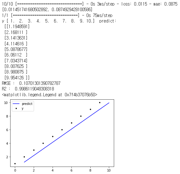
matplotlib의 3줄 만으로 위의 그래프를 그릴수 있다.
import matplotlib.pyplot as plt
plt.plot(x, predict, 'b', x, y, 'k.')
plt.legend(['predict', 'y'])
plt.plot(x, predict, 'b', x, y, 'k.')
plt.legend(['predict', 'y'])
plt.plot(x, predict, 'b', x, y, 'k.')에서 두개의 그래프를 그리고 있다.
x와 predict 값으로 파란색 'b' 라인을 그린다.
x와 y 값으로 검은색 'k.' 점을 그린다.
plt.legend(['predict', 'y'])
범례 'predict', 'y'를 그린다.
참고)
matplotlib에서 여러개의 그래프 그리기
https://dsbook.tistory.com/275